Finding Joint Trajectories to Hit Ping Pong Balls
The Drake KinematicTrajectoryOptimization class can be used to plan robot joint trajectories. These trajectories are represented by the control points of a B-spline. This method of controlling a robot arm is much more powerful than differential inverse kinematics: the method I used to draw laser squares. Chapter 6 of Robot Manipulation has been super helpful in learning about trajectory optimization.
Arm Control Methods
Diff IK uses the pseudo-inverse of the jacobian to control the robot by transforming a desired end-effector velocity into optimal joint velocities. It is good for low-level control, manual jogging, and simple movements, but it has no sense of planning like trajectory optimization. Diff IK can get wonky around singularities, because the inverse jacobian will contain large values that correspond to large joint velocities to achieve much smaller end-effector velocities. Additionally, Diff IK alone only provides information on how the end effector moves relative to the joints for a given pose, and doesn’t take into account velocity or acceleration limits. To move to a constrained Diff IK problem, a quadratic program with linear constraints can be used instead of the simple pseudo-inverse matrix.
Full IK can provide better poses than Diff IK, because it accounts for all possible poses rather than just the end-effector movement relative to it’s current pose. This isn’t to say it always finds the globally optimal pose, but it’s less likely to get stuck at local minimum. However, it also doesn’t guarantee that a small change in end-effector pose will result in a small change in q (the joint positions). For example, at some point when reaching around a pole from the left, it will be more optimal to reach around from the right, and will snap to this new position. Diff IK does not do this because it only describes the velocity of the end-effector for a given pose, it doesn’t search for an optimal position. Often, Full IK is used to find an initial guess for a trajectory optimization program. In my case, this could mean using IK to find a robot pose that meets the ball at the correct position and orientation, and then creating a simple linear B-spline from the start position to the IK solution.
Trajectory optimization can then be used to refine this initial guess, and also constrain the end-effector positions, orientations, and velocities at any point throughout the trajectory, as well as the trajectory length and duration. I don’t believe that trajectory optimization is vulnerable to singularities, because the spline represents joint positions, not end-effector/cartesian positions. One thing I’ve noticed is that some examples of trajectory optimization do not use costs, but the optimization still succceeds. This confuses me, because I would’ve thought that the SNOPT solver would need a cost landscape to descend down. The mysteries of SNOPT…
My Approach
I’ve been working on implementing trajectory optimization on the ping-pong arm. My approach to solving this problem of detecting the ball in flight and finding an arm trajectory to return it was inspired by CatchingBot.
- Given the parametric equations of the ping-pong ball trajectory, I find the time range that the ball will be inside the approximate workspace of the robot.
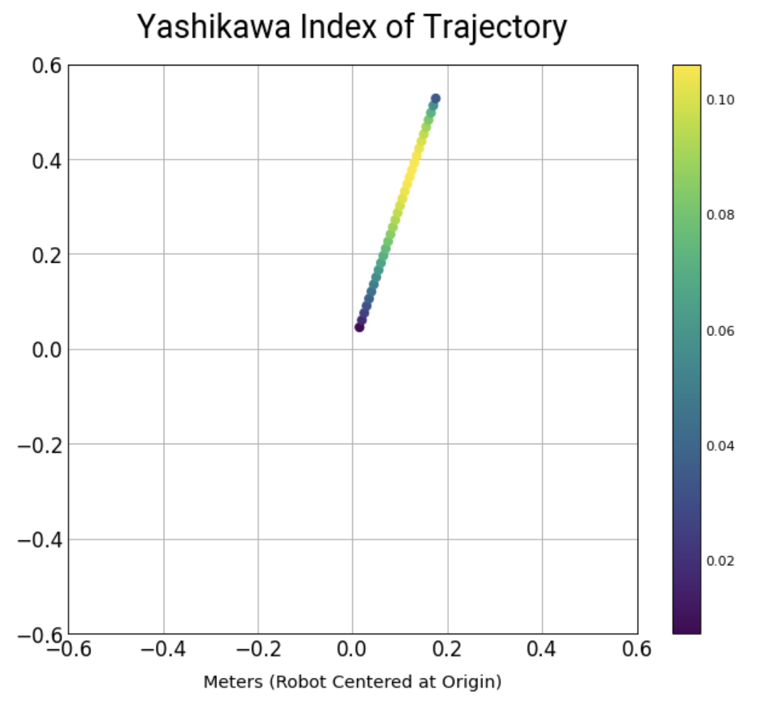
- I sample 50 ping-pong ball poses within this range, and compute robot arm poses via IK that both position the paddle at the ball, and orient the paddle to return the ball to the center of the opposite side of the table.
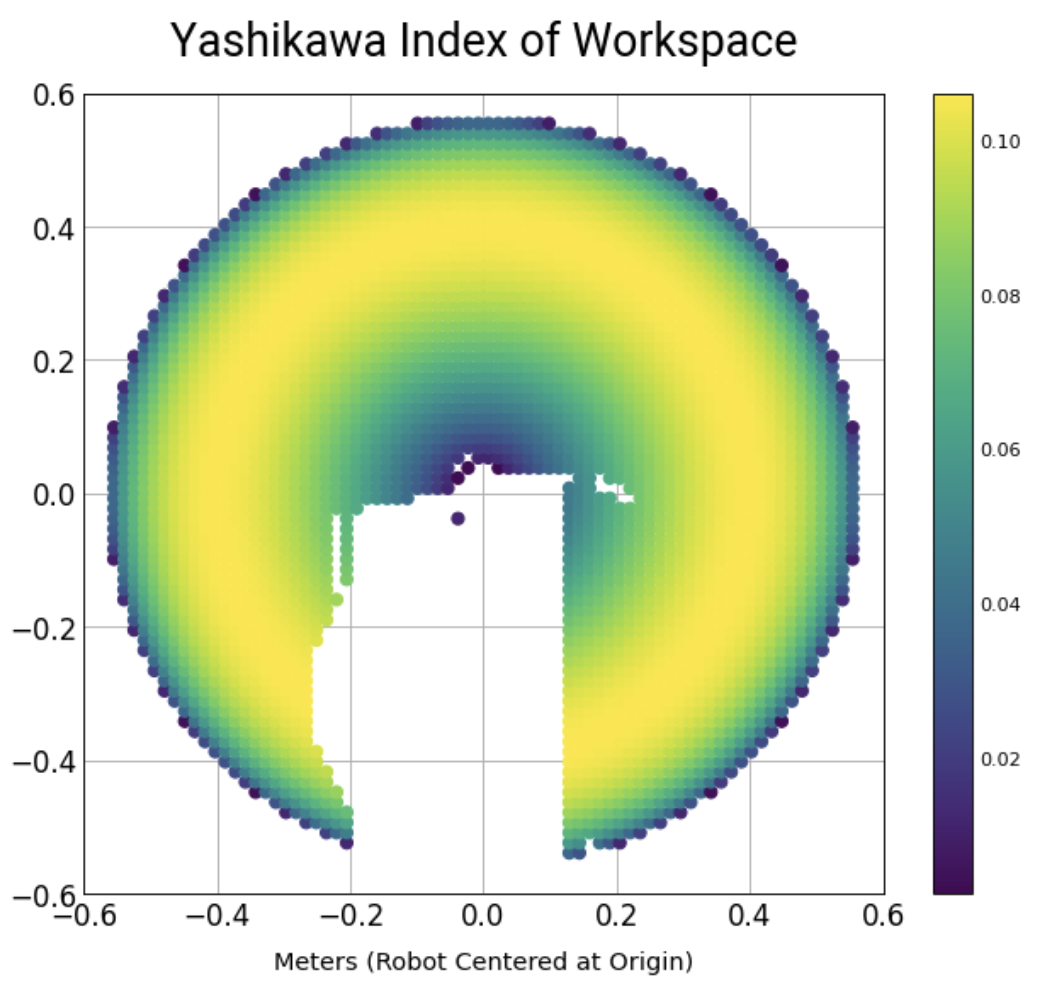
- I score these 50 poses with the Yashikawa manipulation index, \(\sqrt{\det{(J(q)^2})}\). This gives a measure for how far the arm is from any singularities (which would put the arm in a position where it is unable to move in certain directions to respond to changes in the RANSAC ball trajectory estimation).
- Using the best pose, a trajectory optimization is made so that the robot arm reaches the desired pose and orientation at the same time that the ball will arrive at the position.
Additionally, I ran these simulations on the same 2-DOF arm that I used for square drawing. However, achieving the correct paddle orientation is usually impossible with only two joints, so I added a third wrist joint. I may need to add a 4th to allow the arm to tilt the paddle up and arc the ball upwards. However, I would like to keep it as simple as possible to keep the physical robot weight down.
Note that the large gap in coverage of the workspace below is just because the initial condition to the IK problem wasn’t optimal so the solver sometimes failed.
Ball Trajectory Model
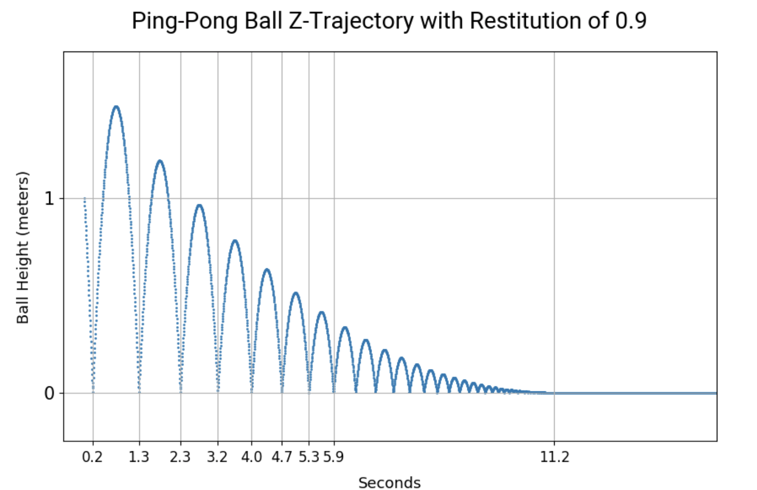
The bouncing ball is represented by three parametric equations, x(t), y(t), and z(t). z(t) is the hardest because in my simple model that doesn’t account for friction/spin/etc, z is the only direction effected by bouncing. This bouncing behavior can be represented by a geometric infinite sequence, where the ratio between terms is the restitution (the bounciness) of the ping-pong ball. Andrew Foote’s blog post was very helpful in creating my model, shown below.
Next Steps
The downside to my approach is that solving these trajectory optimizations is expensive; each one takes about 0.33 seconds. As the ping-pong ball approaches and the RANSAC prediction gets more accurate, I will need a control method that updates the commanded trajectory to respond to these changes in real-time, like with Model Predictive Control. However, MPC is usually used with linearized systems, so I need to figure out how to do that.