SLAM Toolbox Parameters
“SLAM systems require extensive parameter tuning in order to work correctly for a given scenario.” 3
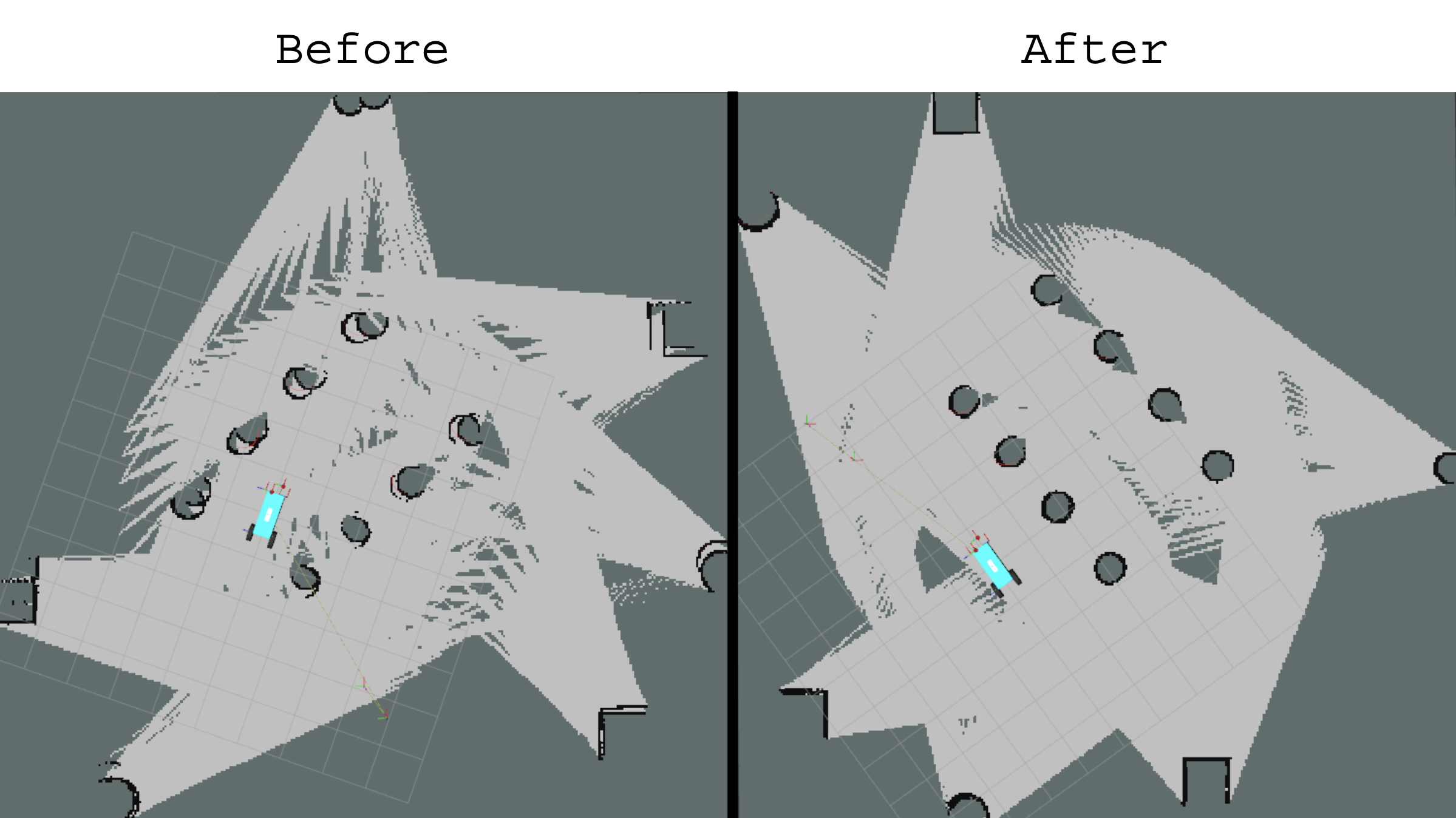
I struggled through this when setting up SLAM Toolbox with Gazebo. Using the default parameters, the algorithm failed to find loop closures in my simulated environment. SLAM Toolbox has well-documented descriptions of each parameter, but given the large number of parameters, I had trouble understanding which parameters to tune first and how changes would affect the end result.
After learning the algorithms used in SLAM Toolbox, I was able to create a cleaner map by tuning the default parameters to my use-case, as shown below.
SLAM Toolbox Parameters Explained
The SLAM node is subscribed to the /tf topic, where it listens for transforms from odom_frame -> base_frame provided by a seperate odometry node. For me, I’m using the ekf_node provided by the robot_localization package, which takes in IMU and wheel encoder measurements to estimate the robot’s position.
Frame Ordering: slam_toolbox orders its frames to follow REP105. Because tf2 requires that transforms be connected in a tree, the base_frame cannot have two parents (map and odom). This also intuitively makes sense; if we want to use forward kinematics to calculate the pose of a frame with respect to one of its ancestors, but there are two paths between the two frames, we might have two disagreeing transforms. Instead, a map_frame -> odom_frame transform is created, which can be described as the correction for the drift of the odometry over time. Because the odometry transformations are often published at a much higher rate than the map updates, a second benefit of ordering the frames from map_frame -> odom_frame -> base_frame is that our map_frame -> base_frame now has the benefits of both the fast and continuous odometry updates and the slower non-continuous error-correction benefits provided by the map.
Questions/TODO
- why does the ekf_node need access to the map_frame? this feels like a circular dependency? The tutorial seems to say its ok to have one ekf_node that just performs continuous odometry and publishes odom_frame -> base_frame, and there can be a second ekf_node that accounts for noncontinuous, jumping, global data provided by a map_transform.
This topic is how slam_toolbox recieves the LaserScan messages. These messages have a timestamp.
Questions/TODO
- what if we want to add other sensor data?
These parameters affect when a laser scan is processed and added to the pose graph.
If the time between two scans (retrieved from the timestamp in the messages’ headers) is less than the minimum_time_interval, SlamToolbox::shouldProcessScan returns false and the scan is either not added to the pose graph (asyncronous mode), or not added to the queue to add at to the pose graph (synchronous mode).
The second two parameters are both used in Mapper::HasMovedEnough. This measures position changes between the current candidate pose and the last pose added to the pose graph. These checks are made in the Mapper::Process method, called from SlamToolbox::addScan. If the pose of the robot in the current scan has not moved enough, then the scan will not be added to the pose graph. These checks are not done on the first scan and when starting a new session with an old map.
Tuning
In summary, these parameters limit the number of scans that make it into the pose graph. It is important that nodes in a pose graph are not too close or too far apart, because…
- Insufficient nodes: less chances for loop closure, less matching points in adjacent scans making scan matching harder? increase number of nodes when no loop closures found?
- Excessive nodes: more complex optimization? reduce number of nodes when laggy? optimizer fails?
Questions/TODO
- why square
m_pMinimumTravelDistanceAND the true distance during the comparison, could just compare absolute values? - The documentation mentions that
minimum_time_intervalis for syncronous mode only, but it seems to be used in asynchronous mode too.
Interlude: Explaining MCSM Scan Matching
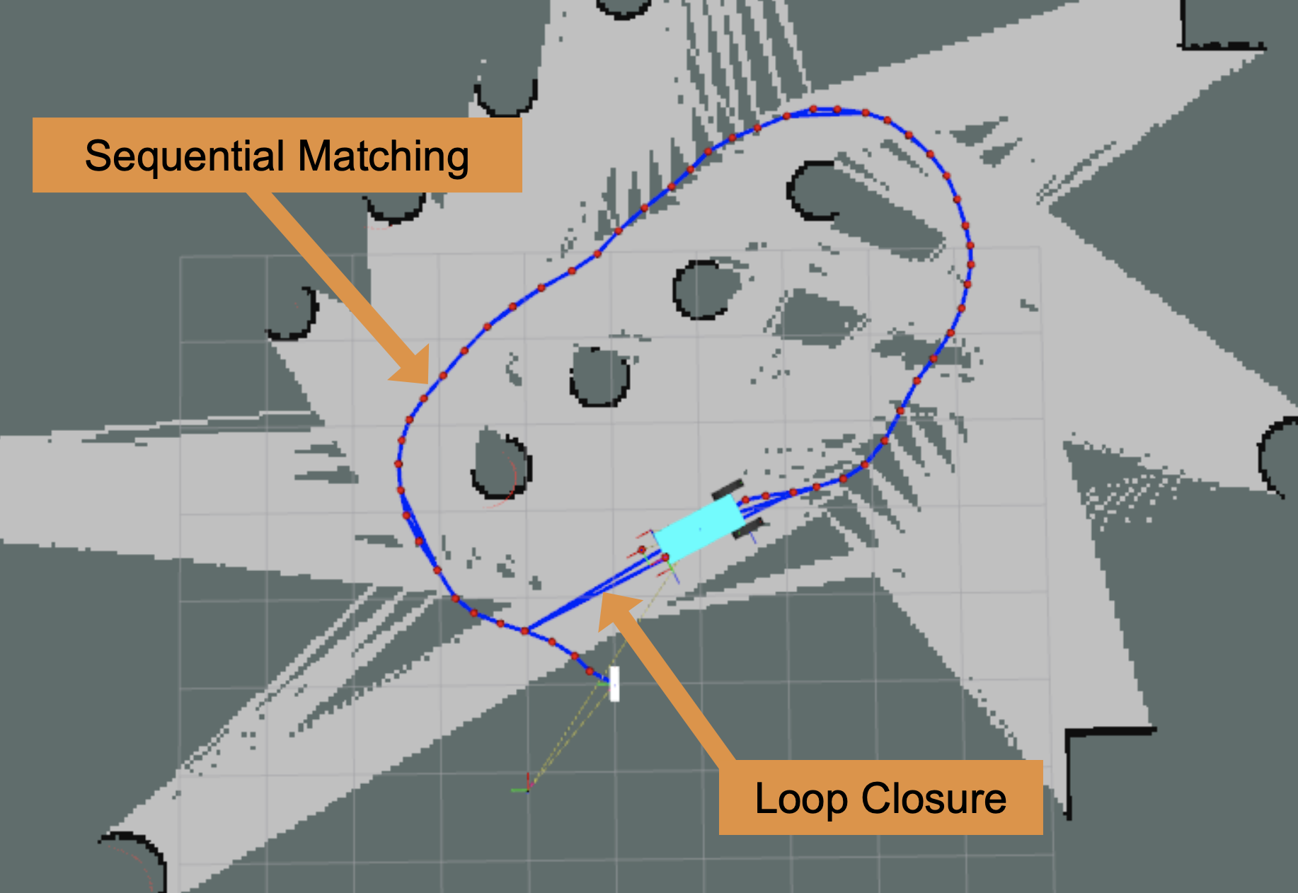
One of the most important part of SLAM algorithms is scan matching: the processes of aligning two pointclouds to determine the transformation (translation and rotation) between them. SLAM Toolbox uses two scan matchers, m_pSequentialScanMatcher and m_pLoopScanMatcher.
The sequential matcher finds transformations between scans taken sequentially, which is used to define edge constraints between nodes in the pose graph and for visual odometry.
The loop matcher searches more broadly for similar scans to close loops when the robot revisits places. These loop closures create edge constriants in the pose graph connecting more distant nodes. Loop closing makes SLAM powerful because it corrects error accumulated over time. Without loop closing, SLAM just becomes a fancy dead-reckoning system.
ICP
ICP is a common point cloud registration technique used in robots. One common ICP use-case is to estimate the pose of a known object in an environment (by matching a model of the object to a lidar or stereo pointcloud of the environment). However, ICP is an iterative optimization technique, and is susceptible to poor initial guesses. In the case of SLAM, if the initial guess provided by wheel odometry and IMU data is inaccurate, it is likely for ICP to get stuck in a local minimum. This is because the cost-landscape of aligning two pointclouds is very non-convex. SLAM Toolbox does not use ICP, but instead MCSM.
CSM (Motion model + Observation model)
CSM (correlation scan matching) and MCSM (muti-resolution auxillary history pointcloud CSM) are more robust point cloud registration techniques used by SLAM Toolbox. Rather than optimizing to reduce the distance between the two pointclouds (ICP), CSM performs a brute-force search over the possible transformations of the scan. This search computes the observation model.
In addition to the observation model, CSM takes into account the robot’s deviation from the initial-guess transformation, where larger deviations are scored worse. For example, if the motor/IMU odometry predicts that the transformation between two scans is an x-offset of 10cm, y-offset of 11cm, and yaw of 4 degrees, transformations near this transformation are scored higher. These odometry measurements inform the motion model.
To paraphrase, CSM has two parts, an observation model and a motion model. It leverages Bayes’ rule to find a probability distribution of the robot’s current position.
\[p(x_i \vert x_{i-1},u,m,z) \propto p(z \vert x_i,m) * p(x_i \vert x_{i-1},u)\]This says that the probability of the robot being at position \(x_i\) (given last position \(x_{i-1}\), motor commands \(u\), map \(m\), and scans \(z\)) is proportional to the observation model * motion model.
- Observation model:
- the probability of observing \(z\) at \(x_i\) in the map \(m\)
- found via scan-matching, better matches have higher probability
- Motion model:
- the probability of the robot being at position \(x_i\) given last position \(x_{i-1}\) and encoder/IMU sensor readings \(u\) (dead reckoning)
- Note: \(u\) is the standard convention representing control inputs. However, I believe it’s used here to represent IMU and wheel encoder sensor data.
Our guess of the current position will be the mean of \(p(x_i \vert x_{i-1},u,m,z)\). However, having the distribution is useful because the variance gives us a confidence interval. Confidence can be encoded into each edge constraint in the pose graph by specifying how “rigid” an edge is during optimization. For example, if the robot is travelling down a hallway that is long in the X direction, it will have more pointcloud points on the nearby walls above and below it in the Y direction. Consequently, it will have high confidence in it’s Y position, and low confidence in it’s X position, as reflected in the covariance.
CSM Brute Search Steps
The process of finding the best translation between a scan and a map via CSM Scan Matching is…
-
User-Specified Inputs
-
Ranges: bounds for x, y, and yaw for maximum translations and rotations
-
Resolutions: step sizes in coarse and fine increments for translations and rotations
-
-
Lookup Table
-
Create a lookup-table using the map, that returns the probability of observing a point existing at some position in the world (high probabilties when near a point in the map)
-
Blur (aka smear) lookup-table to reduce the effects of noisy data
-
Construct a lower-resolution lookup-table via max-pooling. This ensures that the low-resolution map will not miss the best possible high-resolution score
-
-
Coarse Search
-
Use a quadruple for-loop to score all possible translations in the given ranges using the coarse step size
-
The first three for-loops iterate over all possible x, y, yaw transformations
-
The fourth for-loop iterates over each point in the current scan to score via the observation and motion models
-
-
Fine Search
- Using the best transformation from the coarse-search, re-search that coarse pixel using the fine step size
-
Return the best transformation
This method of using both a coarse loop to find the general vicinity of the best transformation, and refining it with a fine loop, is the difference between CSM and MCSM.
CSM Other Notes
-
In the simplest case, the map \(m\)* used for scan matching is just the previous scan. However, multiple previous scans can be combined to increase the pointcloud density, which (1) shows increases accuracy. The number of previous scans used to construct this map can be limited by both a maximum number of scans, or a maximum distance between the current scan and historical scans.
-
To increase the performance of MCSM, (1) recommends keeping the most computationally expensive operation, yaw rotation, in the outermost loop (rotations require trigonometric and multiplicative operations, while translation is only additive).
-
SLAM Toolbox does the outermost loop in parallel:
tbb::parallel_for_each(m_yPoses, (*this)); -
Some papers mention using RANSAC to sample from the map to reduce the effects of outliers, which may be worth experimenting with in noisy environments. Although I imagine it slows down the scan matching because it requires another for-loop to test multiple random samples of the map.
-
I wonder if a hybrid approach could perform better, where a CSM coarse search is used to find a strong initial guess for the ICP algorithm. This might provide more accurate results because the best-possible transformation isn’t limited to the accuracy of the fine resolution step size.
-
Experiments from (2) use a coarse step size of 30cm, and fine step size of 3cm. This 10x multiplier is contrasted by SLAM Toolbox, which only uses a 2x multiplier
- Rotation is coarse to fine:
0.5 * m_pMapper->m_pCoarseAngleResolution->GetValue() - Translation is fine to coarse:
2 * m_pCorrelationGrid->GetResolution()
- Rotation is coarse to fine:
In regards to bullet 2, SLAM Toolbox actually has rotation on the innermost loop (see ScanMatcher::operator()). I believe this is OK because I think SLAM Toolbox uses a larger lookup table with all rotations pre-computed, although I am not sure of this (should study m_pCorrelationGrid and m_pGridLookup for a better answer to this).
These are both used in ScanManager::AddRunningScan to limit the number of scans stored in the std:vector variable m_RunningScans. If there are more than scan_buffer_size scans, or the euclidean distance between the first and last scan is greater than scan_buffer_maximum_scan_distance, the oldest scan is removed.
When a new scan is added and Mapper::Process is called, the m_pSequentialScanMatcher compares the current scan to m_RunningScans (the scans that form the map \(m\)), to find the best pose. Once the best sequential transform has been found and the new node and edges have been added to the pose graph, the current pose is then added to m_RunningScans with ScanManager::AddRunningScan.
Additionally, I think that edges (constraints) in the pose graph are created between the current node, and all nodes from the map \(m\) that were used for scan matching. LinkChainToScan(pSensorManager->GetRunningScans(rSensorName), pScan, scanPose, rCovariance);
Scan matching can also be completely turned of with use_scan_matching. Without this, I cannot get any pose graph to appear on the slam_toolbox/graph_visualization topic, which makes me think a pose graph is not created (even with edges just based on sensor odometry).
In scan matching, the ROS2 LaserScan messages themselves do not form the map and scan. Instead, the messages are transformed into grids, which are cropped and blurred versions of the original messages. This is done in ScanMatcher::AddScan, where the scans are iterated over, and the corresponding cells in the m_pCorrelationGrid are marked as occupied. I think of the correlation grid as a grayscale image aggregation of historical scans. These parameters are used to define the size, resolution, and blurriness of the correlation grid.
When the static method ScanMatcher::Create is called, one of the created member variables is pCorrelationGrid. For the m_pSequentialScanMatcher correlation grid, correlation_search_space_dimension defines the map size (how much cropping is done), and correlation_search_space_smear_deviation describes how much map blurring is done. The other two parameters do the same for the m_pLoopScanMatcher. The number of cells in the grid is not actually ...search_space_dimension itself, but the ...search_space_dimension / ...search_space_resolution (plus some additional padding).
Scan Match Translation Search
As I talked about above, MCSM uses a triple for-loop to loop over the given x, y, and yaw ranges in step sizes based on given resolutions. As you will see in the box below, for yaw, these ranges and resolutions can be explicitly defined by the user. However, for x and y, the range and resolution of the search is determined by the size (...search_space_dimension) and resolution (...search_space_resolution) of the correlation grid itself in ScanMatcher::MatchScan. The coarse resolution is hardcoded to be twice that of the fine resolution.
Questions/TODO
- Why is the correlation grid blurred after each point from a scan is added, and not after all points are added, or even all scans are added?
m_pCorrelationGrid->SmearPoint(gridPoint);
- What is the difference between
pSearchSpaceProbsandpCorrelationGrid? - ScanMatcher::Create is a static class method… why not just use a constructor?
- what is rangeThreshold in
ScanMatcher::Create
These values are used in the yaw for-loop of MCSM to define the range of possible rotations to explore and the step size. The parameters are defined in radians, although I talk in degrees below for simplicity.
-
An offset of 15 degrees would mean poses 15 degrees each way would be scored: a 30 degree range in total.
-
The fine angle step size is hardcoded as 1/2 of
coarse_angle_resolution.0.5 * m_pMapper->m_pCoarseAngleResolution->GetValue() -
If a sufficient match is not found between the scan and map, and
use_response_expansionis set to true, thecoarse_angle_resolutionwill be increased by 20 degrees, and a search will be run again. If a match is still not found, attempts are also made at 40 and 60 degrees. -
Unlike the translational offsets and resolutions, the angle offsets and resolutions are shared between both the sequential and loop matching scan matchers.
Questions/TODO
- what defines a sufficient match? AKA how can the
bestResponsebe 0.0, each translation must have some score. - When running
use_response_expansionloops, maybe add functitionality to not re-search the inner range? - Why is a
fine_search_angle_offsetparameter given? Once a coarse maximum score is found, don’t we know that best score must be somewhere within thecoarse_angle_resolution?- and this is why
fineSearchOffset(coarseSearchResolution * 0.5), aka for translation, the offset is set to the resolution since we know the best score must be within the pixel
- and this is why
During the scoring of transformations within the triple for-loop of CSM, the motion model of the scan matcher penalizes transformations that are further from the inital guess made by odometry.
\[\displaylines { \text{penalty} = 1 - \frac{\text{squaredDistance}}{\text{variancePenalty}} \\ \\ \text{clippedPenalty} = \text{max}(\text{penalty}, \text{minimumPenalty}) \\ \\ \text{score} = \text{observationModelScore} * \text{clippedPenalty} }\]So this penalty is bounded between the minimum and 1 (as long as the variance penalty is not negative), and it scales the response of the score found via scan matching in GetResponse.
This motion model is not used for the loop closure scan matcher (doPenalize is set to false).
Questions/TODO:
- I need to better understand chains
Papers
- Liu, Haiqiao, et al. “Correlation scan matching algorithm based on multi‐resolution auxiliary historical point cloud and lidar simultaneous localisation and mapping positioning application.” IET Image Processing, vol. 14, no. 14, 14 Oct. 2020, pp. 3596–3601, https://doi.org/10.1049/iet-ipr.2019.1657.
- Olson, E.B. “Real-Time Correlative Scan Matching.” 2009 IEEE International Conference on Robotics and Automation, May 2009, https://doi.org/10.1109/robot.2009.5152375.
- Cadena, Cesar, et al. “Past, Present, and Future of Simultaneous Localization And Mapping: Towards the Robust-Perception Age.” IEEE Transactions on Robotics, 19 June 2016.